1. Distribution model

Import the necessary functionalities from Relife

import numpy as np
import matplotlib.pyplot as plt
from relife import Weibull, Gompertz
from relife.datasets import load_circuit_breaker

Here is a toy datasets that contains the following 15 first data

import pandas as pd

time, event, entry = load_circuit_breaker()
data = pd.DataFrame({"time": time, "event": event, "entry": entry})
display(data.head(n=15))

	time	event	entry
0	34.0	1.0	33.0
1	28.0	1.0	27.0
2	12.0	1.0	11.0
3	38.0	1.0	37.0
4	18.0	1.0	17.0
5	32.0	1.0	31.0
6	44.0	1.0	43.0
7	49.0	1.0	48.0
8	27.0	1.0	26.0
9	47.0	1.0	46.0
10	44.0	1.0	43.0
11	70.0	1.0	69.0
12	40.0	1.0	38.0
13	37.0	1.0	35.0
14	26.0	1.0	24.0

1.1. Basics

One can instanciate a Weibull distribution model as follow

weibull = Weibull()

From now, the model parameters are unknow, thus set to np.nan

print(weibull.params_names)
print(weibull.params)

['shape', 'rate']
[None None]

1.2. Parameters estimations

One can fit the model. You can either return a new fitted instance or fit the model inplace

weibull.fit(time, event, entry, inplace=True)
print("Estimated parameters are :", weibull.params)

Estimated parameters are : [3.7267452  0.01232326]

1.3. Plots

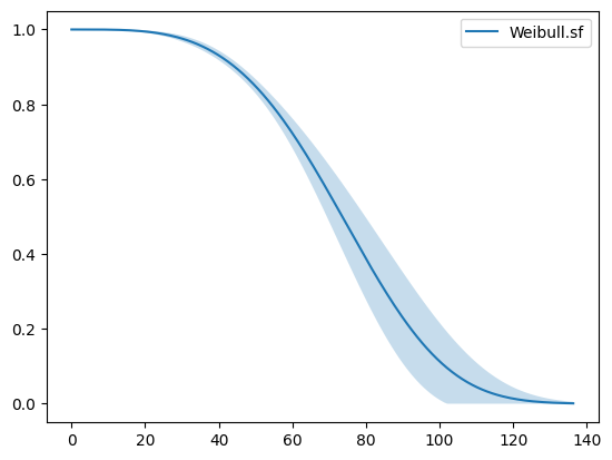
To plot the survival function, do the following

weibull.plot.sf()

<Axes: >